How to Use LiDAR Scans for 3D Crop Canopy Analysis and Yield Forecasting

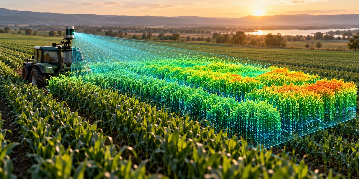
LiDAR technology has moved from autonomous vehicles and forestry surveys straight into the heart of modern crop research. If you have ever tried to estimate canopy volume by hand or relied on NDVI alone, you already know the frustration. A two dimensional snapshot cannot tell you how tall the plants are, how dense the foliage is, or where the biomass is actually concentrated. LiDAR solves that by shooting millions of laser pulses per second and building a precise 3D point cloud of your field. The result is a structural map that lets you measure plant height, leaf angle, canopy porosity, and even predict yield weeks before harvest.

Why LiDAR Beats Other Sensing Methods for Canopy Analysis

Multispectral and RGB cameras measure light reflected from the top of the canopy. They miss everything underneath. LiDAR, whether mounted on a drone, a tractor, or a tripod, sends its own laser energy and records the time it takes to bounce back. That gives you height data from the top of the plant all the way down to the soil.

This vertical resolution matters when you are trying to calculate biomass. A corn field that looks uniformly green from above might have significant gaps in the lower canopy. Those gaps mean less photosynthetic tissue and lower yield potential. LiDAR captures those gaps. It also handles tall crops like sorghum or industrial hemp better than photogrammetry, which struggles with repetitive texture and wind movement.

For researchers running variety trials, LiDAR data can separate subtle differences in plant architecture that correlate strongly with final grain weight. If you are comparing two hybrids that look identical from above, a LiDAR scan might show that one has a 15 percent denser mid canopy. That difference often translates directly into bushels per acre.

The Core Workflow for LiDAR Crop Canopy Analysis

Getting usable numbers from a LiDAR scan requires a repeatable pipeline. Here is the process that most precision agronomy teams follow today.

1. Plan the flight or survey path. For drone based LiDAR, set the flight altitude between 40 and 80 meters above ground level. Keep forward overlap above 70 percent and side overlap above 60 percent. This ensures enough point density to resolve individual plants. For ground based scanning, set up a transect pattern that covers at least three representative zones per field.

2. Collect and preprocess the point cloud. Raw LiDAR data comes as .LAS or .LAZ files. Strip out noise from dust, birds, or hardware glitches using statistical outlier removal. Classify the ground points using a progressive morphological filter. Subtract the ground elevation to get normalized height above ground for every vegetation point.

3. Extract structural canopy metrics. From the normalized point cloud, calculate the 95th percentile height (often called canopy height), the leaf area density profile using the Beer Lambert law adapted for LiDAR, and the gap fraction at different vertical layers. These three metrics form the backbone of most yield models.

4. Build a yield forecast regression. Correlate the LiDAR derived metrics against historical harvest data from the same field or from calibration plots. A simple multiple linear regression using mean canopy height and leaf area density often achieves an R squared above 0.8. For more complex canopies like orchards, use random forest or gradient boosted trees.

5. Validate and iterate. Ground truth at least 5 percent of your plots with manual height measurements and destructive biomass samples. Update your model coefficients each season as crop genetics and weather patterns shift.

Key LiDAR Metrics for Yield Forecasting

Not all point cloud statistics are equally useful. The table below shows the most reliable metrics and the common mistakes researchers make when extracting them.

Metric	What It Measures	Common Mistake
Canopy height (95th percentile)	Maximum vegetation height, robust to outliers	Using mean height instead, which gets pulled down by gaps
Leaf area density (LAD)	Amount of leaf material per cubic meter	Applying a single LAD value across the whole field instead of per vertical layer
Gap fraction	Percentage of laser pulses that reach the ground	Forgetting to filter out low intensity returns from soil
Canopy volume	Total 3D space occupied by vegetation	Using convex hull instead of voxel based volume, which overestimates
Vertical distribution ratio	Ratio of upper to lower canopy density	Ignoring the effect of lodging or wind on scan timing

Expert advice: “Do not trust a single LiDAR flight for yield forecasting. Always collect at least two scans during the season: one at early reproductive stage and one at grain fill. The change in canopy volume between those two dates is a stronger predictor of final yield than any single snapshot.” — Dr. Marisol Vega, precision agronomy researcher at University of Nebraska Lincoln.

Choosing the Right LiDAR Platform

Your choice of sensor platform depends on the scale of your operation and the resolution you need.

Drone mounted LiDAR is the most popular option for field scale work in 2026. Sensors like the DJI Zenmuse L2 or the RIEGL miniVUX weigh under a kilogram and integrate easily with sUAS platforms. They deliver 50 to 100 points per square meter at 50 meters altitude. That is enough to resolve individual corn rows and even detect early season weed patches.

Ground based LiDAR (terrestrial laser scanning) provides much higher point density, often exceeding 10,000 points per square meter. This is ideal for research plots where you need to measure individual leaf angles or stem diameter. The trade off is speed. Scanning a single hectare with a tripod mounted system can take an entire day.

Tractor mounted LiDAR is an emerging option for on the go scanning. Sensors mounted on the cab or boom of a sprayer can collect continuous transects as the tractor moves through the field. The data is less dense than drone scans but covers the entire field with minimal extra labor. This approach works well for harnessing farm data to boost crop productivity and efficiency across large acreages.

Processing LiDAR Data Without a Supercomputer

You do not need a $50,000 workstation to process LiDAR point clouds. Open source tools have matured significantly. CloudCompare and PDAL handle the preprocessing steps like noise filtering, ground classification, and height normalization on a standard laptop with 16 GB of RAM. For voxel based volume calculations, try the lidR package in R or the laspy library in Python.

If you prefer a cloud based pipeline, services like Google Earth Engine now accept LAS files and allow you to run structural metric extraction at scale. This is especially useful when you are combining LiDAR data with other sensor layers. For example, you can overlay LiDAR derived canopy height onto harnessing data analytics to improve pest management strategies maps to identify areas where pest pressure correlates with dense foliage.

Common Pitfalls and How to Avoid Them

LiDAR crop canopy analysis is powerful, but it has a learning curve. Here are the mistakes that trip up most newcomers.

Flying too high. Above 100 meters, the point density drops below 20 points per square meter. At that resolution, you lose the ability to distinguish individual plants. You end up with a smoothed surface that looks like a blanket instead of a canopy. Stay below 80 meters for row crops.

Ignoring wind. LiDAR scans a moving target. If wind speeds exceed 10 miles per hour during the flight, the point cloud will show a blurred canopy. The height values become unreliable. Fly only when winds are calm, typically early morning or late evening.

Using the wrong coordinate system. LiDAR data is inherently geographic, but many processing tools expect projected coordinates in meters. If you leave the data in latitude longitude, your volume calculations will be wrong. Reproject to UTM or a state plane system before running any metric extraction.

Overfitting the yield model. It is tempting to throw twenty LiDAR metrics into a machine learning model and hope for the best. That approach often fails when you move to a different field or a different year. Stick to three to five biologically meaningful metrics and validate them with out of sample data.

Integrating LiDAR with Other Precision Ag Tools

LiDAR data becomes even more valuable when you combine it with other layers. Soil sensor maps, for instance, can explain why certain parts of the field have shorter canopies. Weather station data helps you understand whether a low canopy volume is due to genetics or a dry spell during vegetative growth.

If you are already using top strategies for using data analytics to maximize crop yields, LiDAR provides the physical structure layer that those analytics need to make accurate recommendations. Without structural data, your analytics are working blind.

For operations that have adopted how to leverage drone technology for precision farming in 2026, adding a LiDAR payload is a natural next step. The same drone that carries your RGB or multispectral camera can carry a LiDAR sensor on the next flight. The data fusion between the two sensors gives you both the spectral health and the structural form of the crop.

Building a Repeatable LiDAR Survey Protocol

Consistency is the secret to LiDAR success. If you change your flight parameters between seasons, your yield models will break. Here is a simple protocol that works across corn, soybeans, wheat, and cotton.

• Fly at the same time of day for every scan. Solar noon minimizes shadows but increases wind. Early morning offers calmer air but longer shadows. Pick one and stick with it.
• Use the same ground control points every season. Place 5 to 10 reflective targets at known locations around the field. They help you align point clouds from different dates.
• Collect at the same growth stages. For corn, scan at V6, V12, R1, and R3. For soybeans, scan at V4, R1, and R3. These stages capture the most important structural changes.
• Export your metrics in a consistent format. Use a CSV with columns for field ID, date, growth stage, mean canopy height, 95th percentile height, leaf area density, gap fraction, and canopy volume. Append your yield data after harvest.

From Canopy Structure to Yield Forecast

The real payoff comes when you turn LiDAR metrics into actionable yield predictions. The relationship between canopy volume and final yield is not linear across all growth stages, but it is remarkably consistent within a single crop type.

For corn, the peak correlation between LiDER derived canopy volume and yield occurs at the R2 (blister) stage. At that point, canopy volume explains roughly 75 percent of the variability in final grain yield. For soybeans, the best correlation happens at full pod set (R4). For wheat, the boot stage (Feekes 10) gives the strongest signal.

To build your first forecast, take the mean canopy height from your R2 scan and divide it by the historical mean canopy height for that field. Multiply that ratio by your five year average yield. This simple approach gets you within 10 percent of actual yield most years. As you collect more LiDAR seasons, you can refine the model with leaf area density and gap fraction.

The Future of LiDAR in Agriculture

Sensor costs continue to drop. In 2026, a complete drone LiDAR setup costs about the same as a high end sprayer controller. At the same time, processing software is becoming more automated. Several companies now offer turnkey LiDAR analytics that output yield forecast maps directly, without requiring the user to touch a single line of code.

The next frontier is real time LiDAR. Researchers are testing sensors mounted on harvesters that scan the crop milliseconds before the header cuts it. That data could feed yield maps with centimeter level accuracy, replacing the need for weigh pads and moisture sensors.

For now, the most practical path is to start small. Pick one field. Fly it three times during the season. Process the data yourself using open source tools. Compare your LiDAR derived yield forecast to the actual combine yield. Once you see the correlation in your own fields, you will be hooked.

Putting LiDER to Work on Your Farm

LiDAR crop canopy analysis is not a futuristic concept. It is a proven, repeatable methodology that works today. The tools are affordable. The processing pipeline is well documented. And the payoff is a yield forecast that gives you weeks of extra lead time for marketing, storage planning, and input decisions.

Start by identifying a single field that has consistent management history and variety. Fly a LiDAR mission at the reproductive stage. Process the point cloud using the five steps outlined above. Compare the structural metrics to your harvest data. Once you see how tightly canopy volume correlates with yield, you will wonder how you ever scouted without it.

The next season, expand to three fields. Add a second flight at grain fill. Build your own local model. Share your results with the agronomy community. That is how precision agriculture moves from a buzzword to a reliable tool. And it all starts with a few million laser pulses and a willingness to see your crops in three dimensions.